A Deconstruct Note of Machine Learning with Tensorflow

Abstract

This note provide a inside vision of how tensorflow works on Machine Learning processing. We first described how MNIST DataSet implements and it’s data structure, Then we used a classic linear machine method to create a MNIST DataSet based handwritting number recognize application.

I MNIST

MNIST DataSet, As the hello world of Minchine Learning, we usually download it from Yann LeCun’s website (http://yann.lecun.com/exdb/mnist/), and in Tensorflow, MNIST can be easily fetched by follow codes.

The implementations can be checked via function read_data_set at fn read_data_sets(), which accept several parameters.

def read_data_sets(train_dir,
                   fake_data=False,
                   one_hot=False,
                   dtype=dtypes.float32,
                   reshape=True,
                   validation_size=5000,
                   seed=None) -> DataSet:

For the case fake_data == True, it returns a Fake DataSet, DataSet([], [], fake_data=True, one_hot=one_hot, dtype=dtype, seed=seed), otherwise, It will returns the MNIST dataset with a high dimension dataset base.Datasets(train=train, validation=validation, test=test), which include training data:label, validation data:label, and test data:label.

  options = dict(dtype=dtype, reshape=reshape, seed=seed)
  
  train = DataSet(train_images, train_labels, **options)
  validation = DataSet(validation_images, validation_labels, **options)
  test = DataSet(test_images, test_labels, **options)

  # The origin implementation is dirtier than this, there is a pull request
  # https://github.com/tensorflow/tensorflow/pull/10188

And it worth to notify that the fake DataSet is not actuall a Empty DataSet, the fake_data label parameters will cause side-effect of how fn DataSet(fake_data=True).next_batch works.

The above one_hot label means, the labels will be present as `one-hot vertaxs

Lets check about \(Data(image_i)\), You can use matplotlib to display some of them.

import matplotlib as plt
plt.imshow(np.reshape(mnist.train.images[0], (28, 28)), cmap="gray")

%matplotlib inline
import numpy as np
import matplotlib

fig = plt.figure(figsize=(80,80))
for i in range(1, 31):
    img = np.reshape(train_data.images[i-1], (28, 28))
    ax = fig.add_subplot(8, 10, i)
    matplotlib.pyplot.imshow(img, cmap="gray")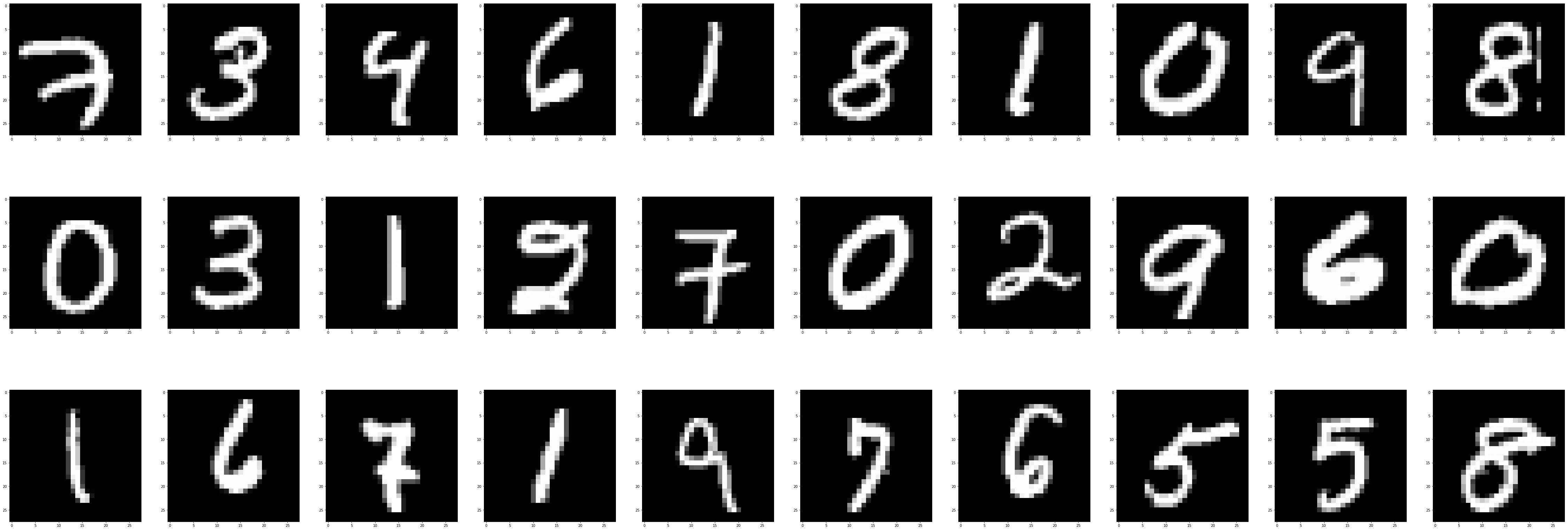

png

All images are shuffled, and you can reshuffle them again by applying function numpy.random.suffle on vetaxs.

II Machine Learning with MNIST via Softmax Regressions

2.1 Linear Regression

Now we have the input image Vertax with 28x28 dimensionals, and needs a function which can map it into a 10 dimensionals Vertax as the one-hot Vertax label. All we needs is to create a Martix with shape (10, 28*28), and a bias. Bias is often used by Term \(linear\ regression\) to refer to a slightly more sophisticated model[5]. Thus the function formula can be descibe as:

Or:

2.2 Multionoulli distribution

Softmax function can be seen as a generalization of the sigmoid function[1], which is also named as logistic function[8] and used to predict the probabilities associated with a multionoulli distribution.

Multinoulli Distribution also knowns as categorical distribution, which is a distribution over a single discrete variable with \(k\) deifferent states, where \(k\) is finite.[2] It’s parametrized by a vector \(P \in [0, 1]^{k-1}\), where \(p_i\) gives the probability of the \(i\)-th state. In this case, \(softmax\) will help us to build a Multinoulli Distribution with a \(k=10\) categorys.

2.3 Implementing with tensorflow

Initialize Vertaxs and Matrixs First:

x = tf.placeholder(tf.float32, [None, 784])

\(x\) is a placeholder of input images which have 28*28 dimensionals.

W = tf.Variable(tf.zeros([784, 10]))
b = tf.Variable(tf.zeros([10]))

Matrix \(W\) and Vertax \(b\) are sets to all Zero.

Thus, We start to implement formule \(f(x)=W^TX+B\) and applied with function \(softmax\):

logits = tf.matmul(x, W) + b
y = tf.nn.softmax(logits)

2.4 Training with Maximum Likelihood Estimation

Machine Leaning is that “\(A\) computer program is said to learn from experience \(E\) with respect to some class of tasks \(T\) and performance measure \(P\), if its performance at tasks in \(T\), as measured by \(P\), improves with experience \(E\) .”by Mitchell(1997).

So, fot training, we needs to find out a method for \(Performance\) measurement, which descript what is good or bad and iterate with optimization \(Task\) and getter \(Experience\) via dataset. Optimization refers to the “task of either minimizing or maximizing some function \(f(x)\) by altering \(x\)”.[4] We usually call the function we want to minimize or maximize as \(cost\ function\), \(loss\ function\) or \(error\ function\).

The Maximum likelihood principle is the most common model for making a good estimater of training models. Consider we have training DataSet $={x_{(1)}, x_{(2)}, , x_{(n)}} $, and a distribute mode \(p_{model}(x;\theta)\) which is based on \(\theta\). The Maximum Likelihood Estimator is defined as:

And we can simply and equivalent trans the product function with sum function:

Ony way to interpret maxium likelihood estimation is to view it as minimizing the dissimilarity between the empirical distribution \(P_{data}\) defined by the training set and the model distribution, weith the degreee of dissimilarity between the two measured by the \(KL\) divergence.

Minimizing this KL divergence corresponds exactly to minimizing the cross-entropy between the distributions.[6]

or

as the documents of tensorflow[4].

2.5 Cross-entropy traing with tensorflow

For cross entropy implementation with Tensorflow, it only needs two lins of code:

y_ = tf.placeholder(tf.float32, [None, 10])
cross_entropy = tf.reduce_sum(tf.nn.softmax_cross_entropy_with_logits(logits=logits, labels=y_))

Then we choosed Grandient Descent Optimizer[7] for minimize cross_entropy:

train_step = tf.train.GradientDescentOptimizer(0.5).minimize(cross_entropy)

2.6 Go Train

Before training start, you may needs to check your hardware resource by code

from tensorflow.python.client import device_lib
device_lib.list_local_devices()

First launch the model session with GPU.

gpu_options = tf.GPUOptions(per_process_gpu_memory_fraction=0.9)
config=tf.ConfigProto(gpu_options=gpu_options, log_device_placement=True)
session = tf.InteractiveSession(config=config)

Then we’ll run the training step 1000 times.

config=tf.ConfigProto(gpu_options=gpu_options, log_device_placement=True)
sess = tf.InteractiveSession(config=config)
tf.global_variables_initializer().run()

for _ in range(1000):
    batch_xs, batch_ys = mnist.train.next_batch(100)
    sess.run(train_step, feed_dict={x: batch_xs, y_: batch_ys})

And Evaluating via below codes:

correct_prediction = tf.equal(tf.argmax(y,1), tf.argmax(y_,1))
accuracy = tf.reduce_mean(tf.cast(correct_prediction, tf.float32))
print(sess.run(accuracy, feed_dict={x: mnist.test.images, y_: mnist.test.labels}))

Reference

[1][2][4][5][6] Book Deep Learning, Author Ian Gooodfellow and Yoshua Bengio and Aaron Courville, MIT Press, page 198

[3][4] MNIST For ML Beginners https://www.tensorflow.org/get_started/mnist/beginners

[7]Machine Learing MOOC, Andrew Ng. https://www.coursera.org/learn/machine-learning/exam/wjqip/introduction